7.1 Introduction
At the time of going to press, satellite surveying relies mainly on a system called global positioning system (GPS), which was originally set up as a military navigation aid by the USA in the mid-1980s, but which has now become a significant tool for civilian use in general and surveyors in particular. Using so-called differential GPS (DGPS), in which data recorded by a receiver at a known station are combined with data recorded simultaneously by a second receiver at a new station which might be 30 km away, it is possible to find the position of the second receiver to within about 5 mm. The advantage of GPS compared to all earlier methods of surveying is that the two stations do not need to have a line of sight between them. This means that national networks of known stations (provided round Great Britain by the Ordnance Survey) no longer need to be located on high hilltops or towers but can, for instance, be positioned on the verges of quiet roads.
7.2 How GPS works
The GPS system consists of a set of about 24 satellites, each of which is in a near-circular orbit about the earth with a period of 12h1 and (therefore) a radius of approximately 26,000 km. The orbits are all inclined at about 55° to the plane of the equator, and lie in six different planes, equally spaced around the equator. As a result, there are at least four satellites visible at all times everywhere on the surface of the earth, unless blocked by terrestrial obstructions. In most places and for most of the time, the number is greater than this, often up to eight or ten. Each satellite broadcasts a set of orbital parameters (the ephemeris) which allow its position at any instant to be calculated to within about 20 m, plus two digital signals whose bits are transmitted at very precise moments in time. By recording the time at which it receives the digital signal (and knowing the speed of light), a GPS receiver is able to determine how far it is away from the satellite (the pseudorange2), and thus to position itself somewhere on a sphere with a known centre and radius.
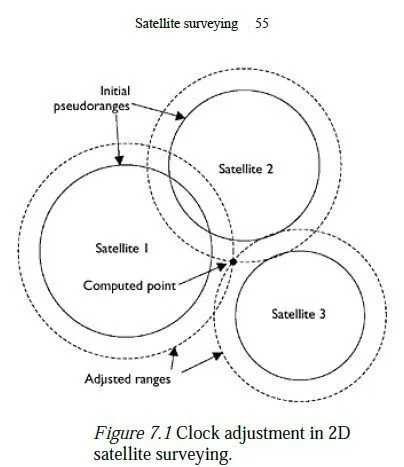
When a second satellite is detected another sphere is calculated, and the locus of possible positions for the receiver becomes the circle of intersection between the two spheres. A third satellite provides another sphere, which will intersect this circle at just two points. One of these will typically lie many thousands of kilometres away from the surface of the earth; discarding this will give one possible position for the receiver. At this point, the principal error in the calculation is caused by the clock in the receiver (the satellites have atomic clocks, which are highly accurate). Because light travels at 300 Mm/s, an error of just 1 μs in the receivers clock will cause an error of 300 m in the calculated radii of all the spheres, and thus a large error in the calculated position. For this reason, a fourth satellite must be detected and a fourth sphere calculated the radii of all four spheres are then adjusted by an equal amount, such that they all touch at one single point. This point is taken as the position of the receiver, and the required adjustment in the radii (divided by the speed of light) is taken to be the receiver clock error. If more than four satellites are visible, the extra information can be used to provide redundancy in the calculation, and the receiver will report a position based on the best fit of the available data. If only three satellites are visible, some systems will also provide a two-dimensional solution, by assuming that the receiver is at sea level. Figure 7.1 is a plan view of the earths surface which shows how three satellites can provide such a 2D solution and correct the receiver clock error. The three solid circles are the loci of all points on the earths surface which are the appropriate distance from each satellite, as calculated from the pseudoranges. As can be seen, there is no one place on the earths surface which lies on all three circles. However, if the receivers clock is running slow, this would cause it to underestimate its distance from each satellite; advancing the receivers clock appropriately and recalculating the ranges gives the three dotted circles, which do meet at a point. The method described above will enable a single GPS receiver to calculate its socalled navigational position to within about 10 m.3 This accuracy can be improved to better than 1 m by leaving the receiver in the same place for an hour or more and averaging the readings. Note that these figures have improved significantly since the US military withdrew selective availability (the deliberate downgrading of the data provided by the satellites) in May 2000 earlier literature quotes much higher errors than this. The accuracy of a result is also determined by other factors, such as the relative positions of the satellites being observed, which will affect the geometry of the computation. This effect is referred to as the geometric dilution of precision (GDOP)4 and is expressed as a multiplying factor for the potential error; a GDOP of less than 2 is very good, but it could rise to 20 or more if all the visible satellites lay in a straight line across the sky. Also, some cheap receivers only use the so-called coarse acquisition (C/A)
digital signals from the satellites to compute pseudoranges, while others also use the more precise P-code, which has a 10-times higher chipping rate.5 Finally, the best receivers are dual frequency they receive the P-code from the satellites on carrier waves at two slightly different frequencies,6 and can thus estimate (and so largely eliminate) the effect of the earths atmosphere on the speed of propagation of the signals. The accuracy discussed above refers to the absolute position of the receiver on the surface of the earth and is considerably higher than anything which could be achieved prior to 1980, using astronomical observations. However, it is insufficient for many engineering purposes, which typically require the differences between stations to be known to a few millimetres. For this reason, surveyors tend to use differential GPS, which is described in the next section.
7.3 Differential GPS (DGPS)
The factors which most affect the accuracy of a single high-quality GPS receiver are errors in the positions of the satellites, errors in the satellite clocks and the effects of the earths atmosphere on the speed at which the satellite signals travel. If two such receivers are within, say, 10 km of each other, the effects of these factors will be virtually identical and the difference vector in their positions will be correct to within a decimetre or two. If the distance between the receivers is greater than this, the accuracy of a simple difference calculation is degraded by the fact that the two receivers will be observing the same satellites, but from somewhat different angles so that the positional and clock errors of the satellites will have slightly different effects on the calculated positions of the two receivers. This is overcome, however, by a more sophisticated form of post-processing which requires one of the receivers to be at a known position, and then effectively corrects the positions of the satellites using the data recorded by that receiver. Ultimately, the accuracy of DGPS is limited by the fact that signals to the two receivers are passing through different parts of the earths atmosphere and will suffer different propagation effects. This constrains the overall accuracy of DGPS to about 2 mm for every kilometre of separation between the two receivers (i.e. 2 parts per million), up to the point where the two receivers can no longer see the same satellites. The final precision of DGPS is achieved by measuring the phase of the carrier wave onto which the P-code is modulated. The chipping rate of the P-code is 10.23 MHz, which means the bits in the signal are about 30 m apart. By contrast, the L1 carrier wave has a frequency of 1,575.42 MHz, and thus a wavelength of about 19 cm. Interpolation of the phase of the carrier signal will yield a differential positional accuracy of a few millimetres, provided it has been possible to use the P-code to obtain a result to within 19 cm beforehand. If not, the carrier phase cannot be used because of the uncertain number of whole wavelengths between the satellite and the receiver. The attempt to determine the number of whole carrier wavelengths is called ambiguity resolution. It is usually possible to resolve ambiguities when the receivers are up to 20 km apart, given a good GDOP and enough observation time and it is usually unwise to attempt it7 if the receivers are more than 30 km apart, because of the unknown differences in atmospheric delays along the two paths. Note, therefore, that the term DGPS can imply a wide range of relative positioning accuracy, from about 2 mm up to 2 dm or so. A final factor which is important at the top level of precision is multipath, i.e. the reception of signals which have not come directly from the satellite but which have bounced off (for instance) a nearby building; this can cause errors of up to half a metre in the calculated position of the receiver. For this reason, differential GPS stations should always be sited well away from buildings and large metal objects. In particular, differential GPS cannot be relied upon to produce accurate results in the middle of a construction site; it is much better practice to use DGPS to fix control stations around the edge of the site, and then to use the more conventional surveying methods within the site.
Base stations for differential GPS
As explained above, if two receivers are more than about 10 km apart, the accurate computation of a DGPS difference vector requires that the absolute position of the base station is known to an accuracy of about 1 m. If a completely local co-ordinate system is to be used for a project, it is perfectly acceptable to base the whole system on a point which has been fixed as a navigational solution, provided it is observed for long enough to fix it to that accuracy. All difference vectors built out from that point will be of high accuracy, and all points fixed using those vectors will also have an absolute accuracy of less than 1 m, so in turn they can be used as base points for further vectors. Often, however, it is necessary to tie in new GPS stations to a countrys national mapping system. This can be done in three different ways, using three different types of known station:
1 Passive stations Most countries, including the UK, provide a network of stations with
known (and published) co-ordinates. These are often sited on roadsides or other public
places, and so can be occupied without obtaining permission. Using one or
(preferably) more of these stations as base stations will tie all new stations into the
national co-ordinate system.
2 Active stations In addition to passive stations several organisations maintain active
base stations at known positions. These record GPS data which are subsequently
published (usually via the Internet) and which can be downloaded for post-processing
in conjunction with data recorded by a roving receiver. This system allows users with
only one GPS receiver to carry out differential GPS and increases the productivity of
users with more than one receiver. The format of the data is normally Receiver-
INdependent EXchange (RINEX), which is the standard format for passing GPS
observations between different manufacturers equipment.
Before using this service, it is wise to check the frequency at which the chosen
active station records its observations (typically once every 15 s), and to set your
own receiver to record at the same frequency; this simplifies and improves the
quality of the subsequent post-processing. Be prepared also to return from
recording your own observations only to find that they cannot be used because the
active station was not working that day!
The fact that the base and the roving station may be using different types of
antenna may also cause problems, as they will have different offsets. The
documentation for the post-processing software should explain how to allow for
this but any error in inputting this information will potentially go undetected. As
a check, download some further data from another active station, with yet another
antenna type, and check that the two differential vectors produce consistent
results.
3 Broadcasting stations An emerging service in several countries is the permanent
installation of GPS receivers which act as base stations and broadcast their data via
short-wave radio to any nearby GPS receiver. Surveyors who have paid to use the
service, and who have suitably equipped receivers, can use this information to show
their position to within a centimetre or so in real time (see Real time kinematic). This
system is also used at airports, enabling DGPS to be used as a precision landing aid.
7.4 Using DGPS in the field
Differential GPS relies on the same satellites being observed at the same time by the two
receivers. If one receiver is recording while the other is not, those observations will be
unusable. There are a number of ways of using DGPS in practice, depending on the size
and purpose of the survey. The principal ones are as follows:
1 Static When the two receivers are more than about 15 km apart, it is necessary for them
to remain simultaneously in position for an hour or more, recording observations every
15 s or so. The time period allows the satellites to move through significant distances
and for a larger number of satellites to be observed by both receivers simultaneouslyand
the number of observations ensures a good chance of resolving ambiguities if that
is desirable or of obtaining a well-averaged result if it is not. Static survey is usually
used for the establishment of new control stations in an area well away from any
existing known stations.
2 Rapid static If the distance between the receivers (the baseline) is less than 15 km, the
observing time can be reduced because the atmospheric effects will be nearly identical
for each receiver. The time required depends on the length of the baseline, the number
of satellites, the GDOP and the algorithms in the receiver. The instruction manual
should give advice on the observation time required; failing that, about 10 min is
probably prudent in most cases. With lines shorter than 5 km, five or more satellites
and a GDOP of less than 8, 5 min will probably be adequate.
3 Stop and go In this procedure, the roving receiver makes a rapid static fix at its first
station and is then moved to other stations while maintaining lock on the satellites
which it is observing. Subsequent points can then be fixed very quickly, in about 10s.
This procedure is suitable for collecting the positions of a large number of points in
open country, but if fewer than four satellites can be tracked at any point, a new
chain must be started by doing another rapid static fix.
4 Kinematic This procedure also starts with a rapid static fix,8 after which the roving
receiver moves continuously, recording its position at regular time intervals (perhaps
as frequently as once per second). As with stop and go, satellite lock must be
maintained at all times. This technique is typically used for surveying boundaries and
other line features.
5 Real time kinematic (RTK) If two suitably equipped receivers are less than about 5 km
apart and have a near line of sight between them, it is possible for the base station to
transmit its position and observations to the roving receiver using a short-wave radio.
The roving receiver can then carry out the DGPS calculations in real time and display
its current position in the GPS co-ordinate system (see Section 7.6). If a suitable
transform has also been downloaded, the roving receiver can also display its position in the local co-ordinate system. Using RTK, the operator of the roving station can
be confident that enough observations have been recorded to resolve ambiguities
while still out in the field, and so can carry out rapid static or stop and go
procedures more quickly. In addition, RTK can be used to set out a station at a
predetermined location, albeit without any independent check of its accuracy
see the next section.
Whichever method is used, there are some fundamental rules which should be followed
when using GPS to maximise the chances of accurate results:
1 Avoid using satellites which are at a low elevation (less than 15° above the horizon,
say), as the signals from these satellites will be greatly affected by atmospheric effects,
due to their long path through the atmosphere. Most surveying GPS systems will
ignore all such satellites, by default.
2 Avoid working close to large buildings. In the northern hemisphere, a building to the
south will tend to block out visible satellites completely, while buildings anywhere
else may cause multipath effects. The combination of these two effects is potentially
disastrous!
3 Working beneath the canopy of a tree can also block the signals from satellites. When
working in stop and go or kinematic mode, just passing briefly beneath the canopy of
a tree can cause loss of lock, resulting in greatly reduced accuracy for all subsequent
readings in the chain.
4 Most GPS processing software allow a surveyor to check in advance what the GDOP of
the satellite constellation will be at the time when it is planned to take readings. This
simple precaution can avoid long periods wasted out in the field, waiting for the
GDOP to improve to the point where useful readings can be taken.
Building a network of stations
Usually, the goal of a GPS survey is to establish the precise location of a number of fixed stations in the field. Logically, this is achieved by fixing the position of an unknown station with respect to a known one using DGPS. The unknown point then becomes known and can be used (if required) as the basepoint for further DGPS vectors, to find the position of other unknown points. In practice, there is no need for the sequence of observations to follow this logical order; it is simply necessary for the results to be processed in that order. Nor is it necessary for one receiver always to act as the base station, while the other always acts as the roving station; it is quite permissible for them to leapfrog each other, taking the role of base and rover respectively as a chain of points is visited. It is, however, important to plan in advance what readings need to be taken, and then to plan a sequence of movements for the receiver(s) to ensure that they are, in fact, taken. A clear written record of what observations have been taken by each receiver (together with a note of the height of the antenna above the station) will also greatly simplify the subsequent processing and archiving of the data. A form for this purpose is given in Appendix G.
7.5 Redundancy
Attentive readers of this book will be aware of the need for redundancy in all surveying measurements. Although properly post-processed differential GPS results are the average of many individual observations, there is still the possibility of a systematic error (one receiver not being in exactly the correct place, for example) which will cause an erroneous result. The straightforward solution to this is to establish each new station by setting up DGPS vectors from at least two known stations. A gross error will then quickly be detected if the two vectors do not meet at almost the same point. Furthermore, the postprocessing software supplied with the GPS equipment will probably contain a leastsquares adjustment facility, which will find a best position for each unknown point, based on the co-ordinates of the known points and the DGPS vectors which have been collected. Clearly, collecting more redundant vectors will result in a more accurate result with a smaller chance of an undetected gross error. If time is limited, redundancy can be achieved by conducting a GPS traverse, similar to the conventional traverse described in Chapter 2. The first unknown point is fixed with respect to an initial known station and is then used to fix the next point. This then becomes the base station for the third point, etc., finally finishing on another known point (preferably not the one where the traverse started). If the position of the final point as calculated by the traverse is in good agreement with its known position, it can be assumed that all has gone well. This approach does, however, have two drawbacks: 1 It is possible that a satisfactory result masks two errors which have cancelled out, e.g. the incorrect entry of an antenna offset when the antenna is used an equal number of times as back station and front station along the traverse. 2 If an error is detected, it will not be possible to determine the leg in which it occurred, and another visit to the site will be necessary. It may, therefore, be wiser to take more redundant readings on the first visit, since this could allow a faulty reading to be eliminated without another site visit. Ultimately, though, all surveyors should be aware that GPS has the tendency to be a black box science, in which a large amount of information is collected and may not be fully checked by the user. There is a distinct possibility of some overall systematic error in the collection or processing of GPS information (the inappropriate use of a program, the wrong settings in a transformation, or a software bug, perhaps) which might cause a completely undetected error in the final result. If absolute confidence is required in a set of new stations for a major project, it is strongly advised that a few checks are made by conventional surveying techniques. The re-measurement of some distances using EDM, for example, is generally less accurate than DGPS but will clearly show if a scaling error has inadvertently been introduced into the GPS results. This is simply the modern equivalent of the old practice of pacing a distance which has been measured by tape, to check that the number of complete tape lengths has not been miscounted. Height information obtained from DGPS needs particular care, partly because it is less accurate anyway and partly because of the nature of the co-ordinate system used by GPS, which is described in the next section. If the heights of stations fixed by GPS are to be relied upon, it is strongly recommended that the relative heights of some stations in the network are checked by conventional means, such as levelling (Chapter 6) or by reciprocal vertical angles (Chapter 12). Again, these conventional methods may be less accurate than GPS but if any discrepancies are too large to be accounted for by their inaccuracy, then there is clearly a problem with the GPS results.