It is customary practice to use curved surfaces of failure for determining the passive earth pressure P on a retaining wall with granular backfill if § is greater than 0/3. If tables or graphs are available for determining K for curved surfaces of failure the passive earth pressure P can be calculated. If tables or graphs are not available for this purpose, P can be calculated graphically by any one of the following methods.
1 . Logarithmic spiral method
2. Friction circle method
In both these methods, the failure surface close to the wall is assumed as the part of a logarithmic spiral or a part of a circular arc with the top portion of the failure surface assumed as planar. This statement is valid for both cohesive and cohesionless materials. The methods are applicable for both horizontal and inclined backfill surfaces. However, in the following investigations it will be assumed that the surface of the backfill is horizontal.
Logarithmic Spiral Method of Determining Passive Earth Pressure of Ideal Sand
Property of a Logarithmic Spiral
The equation of a logarithmic spiral may be expressed as
In Fig. 11.23a O is the origin of the spiral. The property of the spiral is that every radius vector such as Oa makes an angle of 90°-0 to the tangent of the spiral at a or in other words, the vector Oa makes an angle 0 with the normal to the tangent of the spiral at a.
Analysis of Forces for the Determination of Passive Pressure Pp
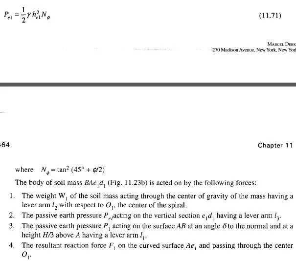
Fig. 1 1 .23b gives a section through the plane contact face AB of a rigid retaining wall which rotates about point A into the backfill of cohesionless soil with a horizontal surface. BD is drawn at an angle 45°- 0/2 to the surface. Let Ol be an arbitrary point selected on the line BD as the center of a logarithmic spiral, and let O}A be the reference vector rQ. Assume a trial sliding surface Aelcl which consists of two parts. The first part is the curved part Ael which is the part of the logarithmic spiral with center at Ol and the second a straight portion elcl which is tangential to the spiral at point e{ on the line BD. e^c\ meets the horizontal surface at Cj at an angle 45°- 0/2. Olel is the end vector rt of the spiral which makes an angle 6l with the reference vector rQ . Line BD makes an angle 90°- 0 with line ^Cj which satisfies the property of the spiral. It is now necessary to analyze the forces acting on the soil mass lying above the assumed sliding surface A^jCj. Within the mass of soil represented by triangle Belcl the state of stress is the same as that in a semi-infinite mass in a passive Rankine state. The shearing stresses along vertical sections are zero in this triangular zone. Therefore, we can replace the soil mass lying in the zone eldlcl by a passive earth pressure Pd acting on vertical section eldl at a height hgl/3 where hg] is the height of the vertical section e{d{ . This pressure is equal to
Determination of the Force P1 Graphically
The directions of all the forces mentioned above except that of Fl are known. In order to determine the direction of F, combine the weight W{ and the force Pel which gives the resultant /?, (Fig. 1 1.23c). This resultant passes through the point of intersection nl of W{ and Pel in Fig. 1 1.23b and intersects force P{ at point n2. Equilibrium requires that force F{ pass through the same point. According to the property of the spiral, it must pass through the same point. According to the property of the spiral, it must pass through the center Ol of the spiral also. Hence, the direction of Fj is known and the polygon of forces shown in Fig. 1 1 .23c can be completed. Thus we obtain the intensity of the force P} required to produce a slip along surface Aelcl .
Determination of P1, by Moments
Force Pl can be calculated by taking moments of all the forces about the center O{ of the spiral. Equilibrium of the system requires that the sum of the moments of all the forces must be equal to
zero. Since the direction of Fl is now known and since it passes through Ol , it has no moment. The sum of the moments of all the other forces may be written as
Pl is thus obtained for an assumed failure surface Ae^c^. The next step consists in repeating the investigation for more trial surfaces passing through A which intersect line BD at points e2, e3 etc. The values of Pr P2 P3 etc so obtained may be plotted as ordinates dl d{ , d2 d’2 etc., as shown in Fig. 1 1 .23b and a smooth curve C is obtained by joining points d{ , d’2 etc. Slip occurs along the surface corresponding to the minimum value P which is represented by the ordinate dd’. The corresponding failure surface is shown as Aec in Fig. 1 1.23b.