In the method of joints, the axial forces in the members of a statically determinate truss are determined by considering the equilibrium of its joints. Since the entire truss is in equilibrium, each of its joints must also be in equilibrium. At each joint of the truss, the member forces and any applied loads and reactions form a coplanar concurrent force system (see Fig. 4.14), which must satisfy two equilibrium equations, ∑Fx =0 and ∑Fy =0, in order for the joint to be in equilibrium. These two equilibrium equations must be satisfied at each joint of the truss. There are only two equations of equilibrium at a joint, so they cannot be used to determine more than two unknown forces.
The method of joints consists of selecting a joint with no more than two unknown forces (which must not be collinear) acting on it and applying the two equilibrium equations to determine the unknown forces. The procedure may be repeated until all the desired forces have been obtained. As we discussed in the preceding section, all the unknown member forces and the reactions can be determined from the joint equilibrium equations, but in many trusses it may not be possible to find a joint with two or fewer unknowns to start the analysis unless the reactions are known beforehand. In such cases, the reactions are computed by using the equations of equilibrium and condition (if any) for the entire truss before proceeding with the method of joints to determine member forces.
member forces. To illustrate the analysis by this method, consider the truss shown in Fig. 4.16(a). The truss contains five members, four joints, and three reactions. Since m+r=2i, the truss is statically determinate. The free-body diagrams of all the members and the joints are given in Fig. 4.16(b). Because the member forces are not yet known, the sense of axial forces (tension or compression) in the members has been arbitrarily assumed. As shown in Fig. 4.16(b), members AB;BC, and AD are assumed to be in tension, with axial forces tending to elongate the members, whereas members BD and CD are assumed to be in compression, with axial forces tending to shorten them. The free-body diagrams of the joints show the member forces in directions opposite to their directions on the member ends in accordance with Newtons law of action and reaction. Focusing our attention on the free-body diagram of joint C, we observe that the tensile force FBC is pulling away on the joint, whereas the compressive force FCD is pushing toward the joint. This e¤ect of members in tension pulling on the joints and members in compression pushing into the joints can be seen on the free-body diagrams of all the joints shown in Fig. 4.16(b). The free-body diagrams of members are usually omitted in the analysis and only those of joints are drawn, so it is important to understand that a tensile member axial force is always indicated on the joint by an arrow pulling away on the joint, and a compressive member axial force is always indicated by an arrow pushing toward the joint.
The analysis of the truss by the method of joints is started by selecting a joint that has two or fewer unknown forces (which must not be collinear) acting on it. An examination of the free-body diagrams of the joints in Fig. 4.16(b) indicates that none of the joints satisfies this requirement. We therefore compute reactions by applying the three equilibrium equations to the free body of the entire truss shown in Fig. 4.16(c), as follows:
Having determined the reactions, we can now begin computing member forces either at joint A, which now has two unknown forces, FAB and FAD, or at joint C, which also has two unknowns, FBC and FCD. Let us start with joint A. The free-body diagram of this joint is shown in Fig. 4.16(d). Although we could use the sines and cosines of the
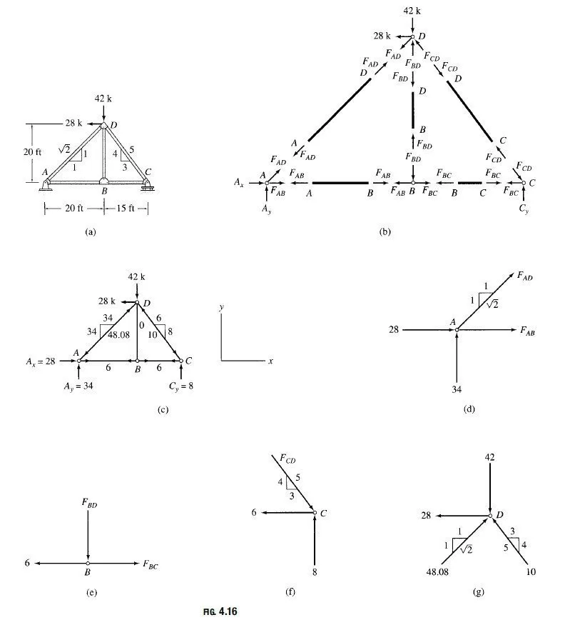
angles of inclination of inclined members in writing the joint equilibrium equations, it is usually more convenient to use the slopes of the inclined members instead. The slope of an inclined member is simply the ratio of the vertical projection of the length of the member to the horizontal projection of its length. For example, from Fig. 4.16(a), we can see that member CD of the truss under consideration rises 20 ft in the vertical direction over a horizontal distance of 15 ft. Therefore, the slope of this member is 20:15, or 4:3. Similarly, we can see that the slope of member AD is 1:1. The slopes of inclined members thus determined from the dimensions of the truss are usually depicted on the diagram of the truss by means of small right-angled triangles drawn on the inclined members, as shown in Fig. 4.16(a).
Refocusing our attention on the free-body diagram of joint A in Fig. 4.16(d), we determine the unknowns FAB and FAD by applying the two equilibrium equations:
Note that the equilibrium equations were applied in such an order so that each equation contains only one unknown. The negative answer for FAD indicates that the member AD is in compression instead of in tension, as initially assumed, whereas the positive answer for FAB indicates that the assumed sense of axial force (tension) in member AB was correct.
Next, we draw the free-body diagram of joint B, as shown in Fig. 4.16(e), and determine FBC and FBD as follows:
In the preceding paragraphs, the analysis of a truss has been carried out by drawing a free-body diagram and writing the two equilibrium equations for each of its joints. However, the analysis of trusses can be considerably expedited if we can determine some (preferably all) of the member forces by inspection that is, without drawing the joint freebody diagrams and writing the equations of equilibrium. This approach can be conveniently used for the joints at which at least one of the two unknown forces is acting in the horizontal or vertical direction. When both of the unknown forces at a joint have inclined directions, it usually becomes necessary to draw the free-body diagram of the joint and determine the unknowns by solving the equilibrium equations simultaneously. To illustrate this procedure, consider again the truss of Fig. 4.16(a). The free-body diagram of the entire truss is shown in Fig. 4.16(c), which also shows the support reactions computed previously. Focusing our attention on joint A in this figure, we observe that in order to satisfy the equilibrium equation ∑Fy =0 at joint A, the vertical component of FAD must push downward into the joint with a magnitude of 34 k to balance the vertically upward reaction of 34 k. The fact that member AD is in compression is indicated on the diagram of the truss by drawing arrows near joints A and D pushing into the joints, as shown in Fig. 4.16(c). Because the magnitude of the vertical component of FAD has been found to be 34 k and since the slope of member AD is 1:1, the magnitude of the horizontal component of FAD must also be 34 k; therefore, the magnitude of the resultant force FAD is FAD =√(34)²+(34)² = 48:08 k. The components of FAD, as well as FAD itself are shown on the corresponding sides of a right-angled triangle drawn on member AD, as shown in Fig. 4.16(c). With the horizontal component of FAD now known, we observe (from Fig. 4.16(c)) that in order to satisfy the equilibrium equation ∑Fx =0 at joint A, the force in member AB ðFABà must pull to the right on the joint with a magnitude of 6 k to balance the horizontal component of FAD of 34 k acting to the left and the horizontal reaction of 28 k acting to the right. The magnitude of FAB is now written on member AB, and the arrows, pulling away on the joints, are drawn near joints A and B to indicate that member AB is in tension. Next, we focus our attention on joint B of the truss. It should be obvious from Fig. 4.16(c) that in order to satisfy ∑Fy =0 at B, the force in member BD must be zero. To satisfy ∑Fx =0, the force in member BC must have a magnitude of 6 k, and it must pull to the right on joint B, indicating tension in member BC. This latest information is recorded in the diagram of the truss in Fig. 4.16(c). Considering now the equilibrium of joint C, we can see from the figure that in order to satisfy ∑Fy = 0, the vertical component of FCD must push downward into the joint with a magnitude of 8 k to balance the vertically upward reaction of 8 k. Thus, member CD is in compression. Since the magnitude of the vertical component of FCD is 8 k and since the slope of member CD is 4:3, the magnitude of the horizontal component of FCD is equal to ð3=4Ãð8à ¼ 6 k; therefore, the magnitude of FCD itself is FCD =√(6)²+(8)² = 10 k. Having determined all the member forces, we check our computations by applying the equilibrium equations PFx ¼ 0 at joint C and ∑Fx = 0 and ∑Fy = 0 at joint D. The horizontal and vertical components of the member forces are already available in Fig. 4.16(c), so we can easily check by inspection to find that these equations of equilibrium are indeed satisfied. We must recognize that all the arrows shown on the diagram of the truss in Fig. 4.16(c) indicate forces acting at the joints (not at the ends of the members).
Identification of Zero-Force Members
Because trusses are usually designed to support several di¤erent loading conditions, it is not uncommon to find members with zero forces in them when a truss is being analyzed for a particular loading condition. Zero-force members are also added to trusses to brace compression members against buckling and slender tension members against vibrating. The analysis of trusses can be expedited if we can identify the zero-force members by inspection. Two common types of member arrangements that result in zero-force members are the following:
1. If only two noncollinear members are connected to a joint that has no external loads or reactions applied to it, then the force in both members is zero.
2. If three members, two of which are collinear, are connected to a joint that has no external loads or reactions applied to it, then the force in the member that is not collinear is zero.
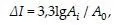
The first type of arrangement is shown in Fig. 4.17(a). It consists of two noncollinear members AB and AC connected to a joint A. Note that no external loads or reactions are applied to the joint. From this figure we can see that in order to satisfy the equilibrium equation ∑Fy = 0, the y component of FAB must be zero; therefore, FAB =0.
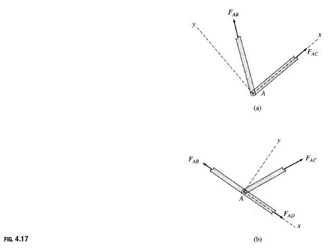
Because the x component of FAB is zero, the second equilibrium equation, ∑Fx =0, can be satisfied only if FAC is also zero. The second type of arrangement is shown in Fig. 4.17(b), and it consists of three members, AB;AC, and AD, connected together at a joint A. Note that two of the three members, AB and AD, are collinear. We can see from the figure that since there is no external load or reaction applied to the joint to balance the y component of FAC, the equilibrium equation ∑Fy = 0 can be satisfied only if FAC is zero.