6.5 Permanent adjustments

The permanent adjustments which can be made to a level ensure that the line of collimation is horizontal when the instrument has been levelled. Alterations to these adjustments should only be undertaken back at base, but it is sometimes useful to check them in the field, particularly if the instrument has just been subjected to a heavy impact.

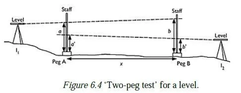
A simple field test called the two-peg test involves driving two pegs into the ground, a measured distance x (usually 25 m) apart, as shown in Figure 6.4. Set the instrument up approximately in line with (but not in between) the two pegs, and observe to the staff on each peg in turn (readings a and b in Figure 6.4). Move the instrument to the other end of the line (so that the peg which was near to the instrument is now the far one) and repeat the process, to obtain readings a² and b². The slope error of the instrument (in radians) is given by the expression ((b−b²)−(a−a²))/2x when all distances are expressed in metres, and a positive value denotes an upward slope. If the absolute value is less than 0.0001, then the instrument is fine; remember that even a value of 0.0002 would cancel completely if the foresights and the backsights are of equal length, and would only produce 1 mm of error if the sight lengths differed by 5 m. For information about tests and adjustments for a particular instrument, refer to the makers handbook. (Some instruments have software for computing the results of a twopeg test automatically.)

6.6 Precision levelling

A slower but much more accurate type of levelling is known as precision levelling, in which differences in heights are typically read to 0.01 mm. The overall principles are identical to those described above, but some extra details are required to achieve the higher precision:

1 The staff is not rocked backwards and forwards as described above, but is supported by some form of tripod and is made precisely vertical by means of a staff bubble. Precision levelling staffs are typically made of Invar, to minimise errors caused by thermal expansion.

2 For maximum accuracy, two staffs are used: one for the backsight and one for the
foresight. Since the staffs may not be identical, it is essential that bays start and end
using the same staff. This means that open bays must always have an even number of
instrument positions. The smallest possible closed bay (from a known benchmark to
a new station and back to the known one) will therefore involve four instrument
positions, so that the same staff is always placed on all the temporary bench marks
which are to be used as the starting point of a new bay. Thus, the bay from A to C and
back in Figure 6.2 would be a valid bay for two-staff precision levelling, but the bay
from C to E and back is too small.
3 The purpose of using two staffs is to allow for changes in temperature which would
cause even an Invar staff to change slightly in length. The procedure is to read a
backsight, then a foresight, then a second foresight and finally a second backsight. The
time interval between readings 3 and 4 is made as close as possible to that between
readings 1 and 2. Averaging the two results eliminates any temperature effects,
assuming that both staffs are heating (or cooling) at a constant rate.
4 The possibility of cumulative errors from a collimation error in the instrument is more
important. To guard against this, the cumulative totals of distances to the backsights
and foresights in a bay are recorded at each step and are kept as close to one another as
possible throughout each bay. The distances are often measured by tachymetry (see
Section 5.2) but can also be taped for maximum accuracy and for planning the layout
of a bay.
5 All modern instruments read the staff electronically, the staff being marked with a bar
coding rather than with numbers. (Older instruments had an optical vernier consisting
of a piece of glass with high refractive index and precisely parallel surfaces, which
made them very expensive.)
6 The importance of finding firm ground on which to stand the staffs is much greater.
The staffs are heavy and may settle by a millimetre or more on soft ground while the
readings are being taken. Even on firm surfaces, it is advisable to let each staff rest for
a minute or so before taking the first reading.

6.7 Contours

Contours (Bannister et al., 1998) are the best method of showing variations in level on a plan; they may be thought of as the tidemarks left by a flood as it falls by successive vertical intervals. Contouring is laborious; the following methods are used:

1 The contours are pegged out on the ground with a level and a staff and then surveyed
(perhaps by a total station). The staff may have a movable vane set at the same height
as that of the telescope above the required contour level, to speed its positioning.
2 A total station is set up and oriented as for mapping (see Section 3.3), above a station of
known height. A detail pole is set to the height of the instrument above its station, so
that any height difference between instrument and reflector is always the same as the
height difference between the station and the foot of the pole. The height difference
from the station to the required contour is calculated, and the pole-holder follows the
ground line which gives this height difference, with the instrument recording the pole position at suitable intervals. The contour is then plotted in the same way as other
mapping detail.
3 The spot levels of points where the slope of the ground changes are taken, usually with
a total station, and the contours are interpolated. This is a common method in
engineering work; it is less accurate than method (2), but much quicker.
4 Heights are measured at evenly spaced points on a (x, y) grid, and the contours are
drawn by interpolation. This method is particularly useful if the volume of earth in an
area needs to be estimated, as part of a mass-haul calculation see Allan (1997) for
details. Some total stations can steer the detail pole to the necessary places and
perform the volume calculations.
5 Over larger areas, contours are most easily plotted by means of aerial or satellite
photogrammetry. Contours on published maps are now generally plotted by digital
photogrammetry (Egels and Kasser, 2001).
6 Contours may very effectively be plotted by kinematic GPS (see Chapter 7).