9.2 Individual projections
There are over 60 different types of projection in use around the world, usually selected to give the least overall distortion in the context of the size, shape and location of the area which is to be mapped. It is beyond the scope of this book to describe all of these to a useful level of detail the reader is referred to Bugayevskiy and Snyder (1995) in the first instance. Four projections will, however, be described in further detail, as they are of particular interest to surveyors around the world.
The Lambert conformal projection
This is a conical projection, as described in Section 9.1, and, as its name suggests, the spacing of the parallels is arranged so as to give maps which are conformal. An ellipsoidal shape and two standard parallels must be specified to define the projection fully. The scale factor of the map is unity on these two parallels; between them it is less than unity (meaning that projected features would be smaller than life size on a full-sized projection), and outside them it is greater than unity. It rises to infinity at the pole which is furthest from the apex of the cone, so this pole cannot be shown on the map. The USA is typically mapped by means of the Lambert conformal projection; the parallels at 33° N and 45° N and the GRS80 ellipsoid4 are normally used when mapping the entire country. Individual states are also mapped using this projection but with different standard parallels, to minimise the distortion in their particular area of interest. As with all conformal projections, there is only one family of geodesics which project as straight lines, in this case, the meridians. All others will project as curves, and allowance for this must be made for large surveys, as described in the next section. Note that there are several other types of Lambert projection. As stated above, cylindrical and azimuthal projections can be seen as special cases of conical projections, so can be classed as Lambert projections; and Lambert projections are sometimes plotted as equal area projections rather than as conformal ones. In addition, the azimuthal versions do not always have the North or South Pole as their central point, but may instead use any other point, specified by its latitude and longitude. In these cases, the earth is treated as a sphere rather than as an ellipsoid to simplify the subsequent computations.
The Mercator projection
The Mercator projection is a conformal cylindrical projection, with the cylinder touching the earth around its equator. The scale factor of the projection is a function of latitude only; it is unity on the equator and rises to infinity at the poles. Normally, therefore, a Mercator projection only shows latitudes up to about ±80°. This projection has the useful property that a straight line drawn between two points on the map cuts each meridian at the same angle; this is a so-called rhumb line, which a navigator could set as a constant compass bearing to travel between the two points. However, rhumb lines are not generally the shortest path between two points, and the corresponding geodesics between the same two points plot as curved lines on the map. A major drawback of this projection is that above latitudes of, say, 40°, the scale factor of the map starts to change significantly with increasing latitude. This makes Arctic countries look much larger than they really are, by comparison with tropical ones, and also means that in a country such as Great Britain, the north of Scotland is plotted at a noticeably larger scale than the south of England.
The transverse Mercator projection
Also known as the Gauss-Lambert projection, this is a conformal version of the transverse cylindrical projection described in Section 9.1 (see Figure 9.3), and is defined by specifying the shape of the ellipsoid, a central meridian and the value of the scale factor along it (known as the central scale factor). Great Britain is mapped using a transverse Mercator projection, for the reasons described in Section 9.1. The Airy 1830 ellipsoid5 is used together with the 2° W meridian, being the meridian which most nearly runs up the middle of the country. If the central scale factor for Britain was set to unity on the central meridian, it would rise to about 1.0008 at the extreme east and west of the country. For making a map of the British Isles, it is desirable to have the scale factor as near to unity as possible over the whole of the mapping area; so the central scale factor is actually defined to be about 0.99966 on the central meridian, rising to about 1.0004 at the extreme east and west of the country. This can best be visualised as having the original cylinder lying slightly inside the central meridian, and cutting through the earths surface about 180 km on either side of it; features between the two cutting lines are reduced in size when projected onto the cylinder, and those outside them are enlarged.
The universal transverse Mercator (UTM) projection
This projection system provides a low-distortion projection of the whole world and consists of separate transverse Mercator projections of 60 so-called zones (segments) of the earths surface, lying between lines of constant longitude. Each zone covers a 6° band of longitude, with zone 1 having its central meridian on the 177° W meridian, and subsequent zones following on in an easterly direction. Thus, the central meridian of zone 29 is 9° W, that of zone 30 is 3° W and that of zone 31 is 3° E. (These are the three zones which are of relevance to the UK.) The central scale factor of each zone is exactly 0.9996. The UTM projection is normally used in conjunction with the international 1924 ellipsoid, whose details are given in Appendix A. However, it is sometimes used in conjunction with other ellipsoids (e.g. WGS84), so it is wise to check which ellipsoid has been used before processing UTM data. UTM is a useful global projection system but it is not a universal panacea, because a region which does not wholly lie within 6° of one of the 60 central medians cannot be properly plotted on a single TM zone. Possible solutions to this are: 1 to extend a zone slightly, so as to include the whole region; 2 to create a non-standard TM projection, by using a different central meridian; 3 to butt two or more neighbouring UTM projections together in the region of interest. Options 1 and/or 2 are feasible solutions to the problem; a UTM can readily be extended by 500 km on either side of the central meridian, so any area spanning up to 1,000 km from east to west can be handled with negligible loss of accuracy. Option 3 is inappropriate for surveying purposes. As shown in Figure 9.5, the boundaries of neighbouring zones (known as gores) are not straight, so can only touch one another at a single latitude. Thus any other point on the common boundary would map to two separate places on the projection, and lines would kink as they passed from one zone to the next.
![]()
9.3 Distortions in conformal projections
Distortions on a conformal map only become obvious to the naked eye about 45° away from the central meridian (or from a standard parallel in the case of a conic projection). However, some distortion of shape or scale is present over virtually the entire projection, so must be taken into account by surveyors. The two important aspects of distortion in a conformal projection are: (a) that the line of sight between two points does not plot as a straight line and (b) that the scale factor varies from point to point. Methods for dealing with both of these are described below.
Curvature of geodesics
When the line of sight between two points is projected onto the surface of the ellipsoid, the resulting line is called a geodesic, which is defined as the shortest line on the surface of the ellipsoid between the two points in question. On a perfect sphere, geodesics are all great circles, with their centres at the centre of the sphere. On an ellipsoid, things are more complex; some geodesics snake slightly between their two endpoints. However, the geodesics between two points with the same longitude always lie on the (elliptical) line of longitude between the points; and for other points less than about 30 km apart, the difference between a geodesic and a great circle is negligible. In conformal conical projections, the only geodesics which remain exactly straight are meridians; in transverse cylindrical projections, they are the central meridian itself, and those geodesics which cross the central meridian at right angles. All others appear to bulge in the direction of higher scale factor, when projected. (The angles which these lines make with other lines they meet or cross are, however, exactly the same as on the earths surface.) The effect of this distortion can be seen by reference to Figure 9.6, which is a transverse Mercator plot of three stations, A, B and C. If a theodolite is set up on station B and stations A and C are observed, the two lines of sight made by the theodolite will plot as the curved lines on the figure. Because these lines in general bulge by different amounts, the angles they make at B with the corresponding straight lines on the projection (labelled t) are different so the angle between the two lines labelled T (i.e. the horizontal angle observed by the theodolite) will be slightly different from the angle ABC as calculated by trigonometry from the (x, y) co-ordinates of A, B and C. The angles between the T lines and their corresponding t lines at a point can be calculated if the shape of the ellipsoid, the projection parameters and the positions of both endpoints are known; this calculation is called a (t−T)7 correction. For the British National Grid (and, by extension, for UTM projections), the calculation is described fully in Ordnance Survey (1950), pp. 1416. For distances of less than 1 km which lie within 200 km of the central meridian, the (t−T) correction is negligibly small. However, over longer distances, or on conformal projections which cover larger areas, it must be taken into account. In Figure 9.7, for example, the 7° W meridian should ideally project as a straight line between the latitudes 50° N and 58° N, since it is a geodesic; in fact, it cuts the 54° N latitude at a point which is about 800 m west of the intercept made by a straight line drawn on the projection between the same endpoints. The (t−T) correction for this line is about 12 minutes at each end of the ray.
![]()
The (t−T) calculation is tedious to carry out by hand and would normally be done by computer, in the context of adjusting horizontal angle observations. A surveyor should ensure that any adjustment software which works with projected (as opposed to geographical) co-ordinates takes account of this correction, before using it for a largescale survey.
Scale factor distortions
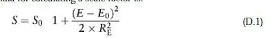
The local scale factor of a projection must be taken into account whenever distances in the field are converted to projected distances. Distances are routinely measured to just a few parts per million, so a local scale factor which lies outside the range 0.999999 1.000001 will make a significant difference. The scale factor of a projection is defined as (projected length/ true length) on the full-size projection so any distance measured on the ellipsoid must be multiplied by the local scale factor before it can be treated as a distance on a conformal projection. (Slope distances or horizontal distances measured above or below the reference ellipsoid require additional processing, as explained in Chapter 11.) In all conformal projections, the scale factor S is a function of the central scale factor (if any) and the distance from the point or line(s) of zero distortion. For short lines (<10 km), the local scale factor will be reasonably constant along the whole length of the line, so a single scale factor can be applied ideally, this would be obtained at the midpoint of the line. For longer lines, the scale factors should be found at both endpoints and at the midpoint of the line; a mean scale factor can then be estimated using Simpsons Rule, i.e.:
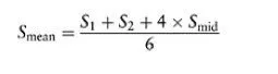
The formula for calculating the scale factor at a point depends on the details of the projection. The formula for calculating scale factors in all transverse Mercator projections is given in Appendix D.