E.1 Bowditch adjustment

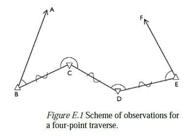
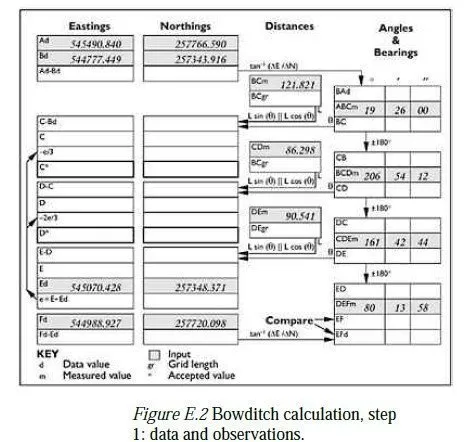
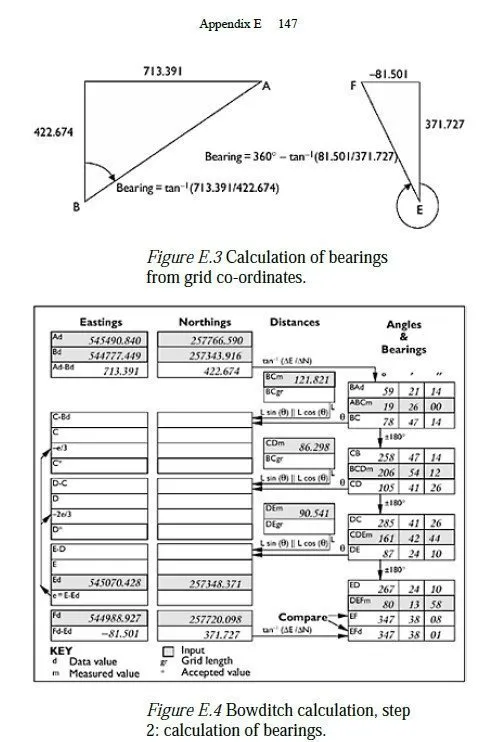
This example shows how the Bowditch calculation sheet, introduced in Chapter 10, is used in a simple traverse to fix the positions of two unknown points (C and D, in Figure E.1). The scheme of observations is as shown in Figure E.1, with stations A, B, E and F having known co-ordinates. Note that this is not a precise drawing but is sketched sufficiently accurately so that the bearings are correct to within 30° or so. It is helpful to make such a sketch before starting the calculations (and even before making the observations) to guard against gross errors. The first stage in the calculation is to transfer the initial data (i.e. the eastings and the northings of the known stations, in the British National Grid) and the observations (i.e. the measured angles and distances) into the shaded boxes on the calculation sheet, as shown in Figure E.2. The next step is to enter the differences in eastings and northings for point A relative to B (Ad-Bd on the calculation sheet) and for point F relative to E (Fd-Ed on the sheet). These are used to work out the bearings from B to A and from E to F. In the case of BA the calculation is straightforward, since A is to the north and east of B, as shown in Figure E.3. For EF the situation is more complex, and a simple sketch like the one shown in Figure E.3 is helpful to make sure that the correct angle is calculated.

Once these bearings have been entered on the sheet (BAd and EFd, respectively), the remaining angle boxes can be filled in. Starting at the top of the right-hand column, the bearing from B to C is calculated by simply adding the measured angle at B to the bearing from B to A. The bearing from C to B is then obtained by adding 180° to this value, since the bearing BC is itself less than 180°. The same process is then repeated to obtain the bearing CD, except that 360° is subtracted from the result to bring it into the range 0360°. The same thing occurs when bearing DE is calculated, and bearing ED is found by subtracting 180° from DE since DE is greater than 180°. Finally, bearing EF is calculated, and the sheet is as shown in Figure E.4. It can be seen that the two calculated bearings for ED (one based on observations and one based purely on data) differ by 7 seconds. This is reasonable; assuming the error of each measured angle has a standard deviation of (say) 5 seconds, the standard deviation of the sum of the four measurements would be 5×√4 seconds.

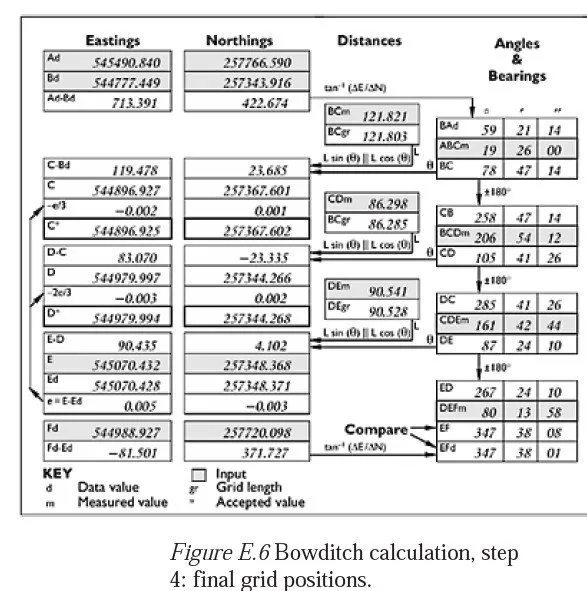
Having passed this test, the calculation moves on to the next stage. The measured horizontal distances are first converted to reduced distances (if necessary), by using equation 11.6, and then to grid distances (if appropriate) by applying the local scale factor.

In this case, the survey is taking place in Cambridge, where heights above sea level are negligible. A scale factor must however be calculated, since the British National Grid is being used; in this case, the size of the traverse means that a single value can be calculated and used for all distance measurements. The survey is less than 200 km from the central meridian, and an accuracy of 2 parts per million will be more than adequate, so equation D.1 can be used.
A suitable mean easting is 545000 m, and E0 and S0 are given in Appendix A. Putting these into equation D.1 gives:

E.2 Leastsquares adjustment

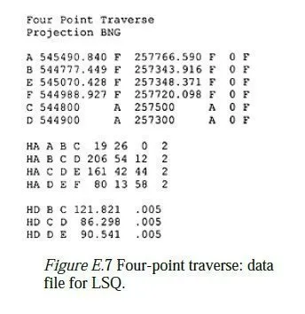
The same adjustment can be done using a least-squares adjustment program, such as LSQ. In the case of LSQ, the data are entered as shown in Figure E.7. The input file follows the rules given in the LSQ help system. The first line is a title and is followed by a line which specifies the projection (in this case, the British National Grid), to enable the local scale factor(s) to be calculated. The next group of lines describes the control stations. Stations A, B, E and F are entered with their known eastings and northings, which are fixed by the letter F which follows them. Stations C and D are given approximate co-ordinates, which are set to be adjustable by the letter A. The heights of all the stations are fixed, as this is a 2D adjustment.

The horizontal angle observations are entered next, in degrees, minutes and seconds; the final number is an estimate (in seconds) of the standard deviation of the error which might be expected in each observation. Two seconds is a typical value for an observation made under favourable conditions with a good quality instrument. The last group of lines records the measured horizontal distances, in metres; again, the final number is the estimated standard deviation (ESD) of the reading. Typically, most EDM devices have a standard deviation of ±5 mm, even on short rays such as these. Running LSQ produces the result shown in Figure E.8, after nine cycles of adjustment. It turns out that this number of cycles is necessary, because of the relatively poor initial guess for the position of C. The co-ordinates which LSQ has chosen for C and D are within 2 mm of those found in the Bowditch adjustment above. These small differences come from the different relative weightings that LSQ is able to give to angle and distance measurements, and from the fact that the Bowditch method only uses the measured angle DEF as a check and not as part of the adjustment. Usefully, LSQ is also able to show the likely accuracy to which C and D have been found, by means of the error ellipses shown on the printout. The major semi-axis of each ellipse is 4 mm, so there is a 95 per cent confidence that C and D lie within 8 mm of their calculated positions (assuming, of course, that the positions of the other points are errorfree).

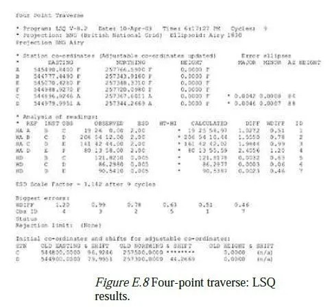
The next block of results compares the readings which were observed with those which would result from the calculated positions of the adjustable points. The differences, or residual errors, are shown both in seconds or in millimetres (as appropriate), and also as weighted differences using the ESD quoted for the reading. Below this the ESD scale factor is shown. This is the calculated standard deviation of the weighted residual errors, and so indicates whether the residual errors are generally bigger or smaller than might have been expected from the quoted ESDs. An ESD scale factor of 2 or more would indicate that either the quoted ESDs were optimistically small, or there are errors other than observation errors in the data. Here, the ESD scale factor looks fine.